Start on TensorBoard

# -*- coding: utf-8 -*-
"""
Created on Tue Mar 22 10:43:29 2016

@author: rob
"""
import numpy as np
import tensorflow as tf
import input_data
from numpy import genfromtxt
sess = tf.InteractiveSession()


#%For quick debugging, we use a two-class version of the MNIST,
#where the targets are encoded one-hot.
# You can use any variation of MNIST. As long as you make sure
#that y_train and y_test are one-hot and X_train and X_test have
#the samples ordered in rows
X_test = genfromtxt('X_test.csv', delimiter=',')
y_test = genfromtxt('y_test.csv', delimiter=',')
X_train = genfromtxt('X_train.csv', delimiter=',')
y_train = genfromtxt('y_train.csv', delimiter=',')

N = X_train.shape[0]
Ntest = X_test.shape[0]

#Check for the input sizes
assert (N>X_train.shape[1]), 'You are feeding a fat matrix for training, are you sure?'
assert (Ntest>X_test.shape[1]), 'You are feeding a fat matrix for testing, are you sure?'
assert (y_train.shape[0]>y_train.shape[1]), 'You are feedinf a fat matrix for labels, are you sure?'

# Nodes for the input variables
x = tf.placeholder("float", shape=[None, 784], name = 'Input_data')
y_ = tf.placeholder("float", shape=[None, 10], name = 'Ground_truth')


# Define functions for initializing variables and standard layers
#For now, this seems superfluous, but in extending the code
#to many more layers, this will keep our code
#read-able
def weight_variable(shape, name):
  initial = tf.truncated_normal(shape, stddev=0.1)
  return tf.Variable(initial, name = name)

def bias_variable(shape, name):
  initial = tf.constant(0.1, shape=shape)
  return tf.Variable(initial, name = name)

def conv2d(x, W):
  return tf.nn.conv2d(x, W, strides=[1, 1, 1, 1], padding='SAME')

def max_pool_2x2(x):
  return tf.nn.max_pool(x, ksize=[1, 2, 2, 1],
                        strides=[1, 2, 2, 1], padding='SAME')

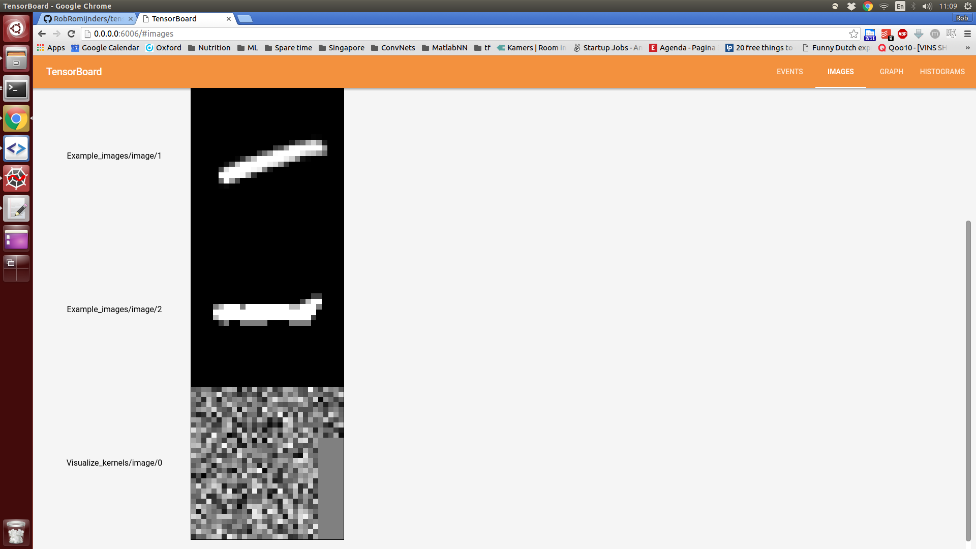
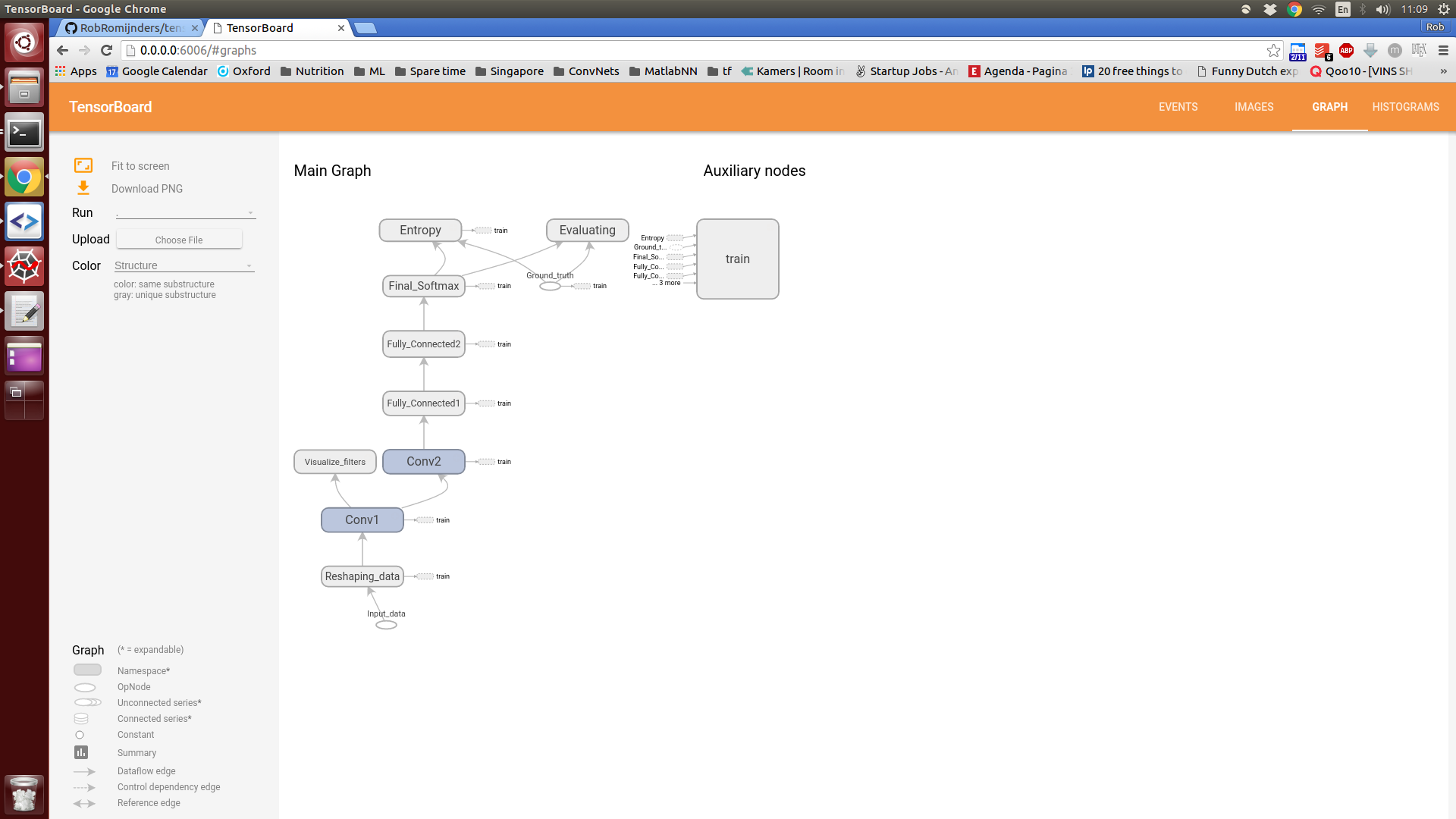
with tf.name_scope("Reshaping_data") as scope:
  x_image = tf.reshape(x, [-1,28,28,1])
  image_summ = tf.image_summary("Example_images", x_image)

with tf.name_scope("Conv1") as scope:
  W_conv1 = weight_variable([5, 5, 1, 32], 'Conv_Layer_1')
  b_conv1 = bias_variable([32], 'bias_for_Conv_Layer_1')
  h_conv1 = tf.nn.relu(conv2d(x_image, W_conv1) + b_conv1)
  h_pool1 = max_pool_2x2(h_conv1)

with tf.name_scope('Visualize_filters') as scope:

# In this section, we visualize the filters of the first convolutional layers
# We concatenate the filters into one image
# Credits for the inspiration go to Martin Gorner
  W1_a = W_conv1                       # [5, 5, 1, 32]
  W1pad= tf.zeros([5, 5, 1, 1])        # [5, 5, 1, 4]  - four zero kernels for padding
  # We have a 6 by 6 grid of kernepl visualizations. yet we only have 32 filters
  # Therefore, we concatenate 4 empty filters
  W1_b = tf.concat(3, [W1_a, W1pad, W1pad, W1pad, W1pad])   # [5, 5, 1, 36]  
  W1_c = tf.split(3, 36, W1_b)         # 36 x [5, 5, 1, 1]
  W1_row0 = tf.concat(0, W1_c[0:6])    # [30, 5, 1, 1]
  W1_row1 = tf.concat(0, W1_c[6:12])   # [30, 5, 1, 1]
  W1_row2 = tf.concat(0, W1_c[12:18])  # [30, 5, 1, 1]
  W1_row3 = tf.concat(0, W1_c[18:24])  # [30, 5, 1, 1]
  W1_row4 = tf.concat(0, W1_c[24:30])  # [30, 5, 1, 1]
  W1_row5 = tf.concat(0, W1_c[30:36])  # [30, 5, 1, 1]
  W1_d = tf.concat(1, [W1_row0, W1_row1, W1_row2, W1_row3, W1_row4, W1_row5]) # [30, 30, 1, 1]
  W1_e = tf.reshape(W1_d, [1, 30, 30, 1])
  Wtag = tf.placeholder(tf.string, None)
  tf.image_summary("Visualize_kernels", W1_e)

# The name_scope lines serve to organize our graphs that TensorFlow will create
# for us
with tf.name_scope("Conv2") as scope:
  W_conv2 = weight_variable([5, 5, 32, 64], 'Conv_Layer_2')
  b_conv2 = bias_variable([64], 'bias_for_Conv_Layer_2')
  h_conv2 = tf.nn.relu(conv2d(h_pool1, W_conv2) + b_conv2)
  h_pool2 = max_pool_2x2(h_conv2)

with tf.name_scope("Fully_Connected1") as scope:
  W_fc1 = weight_variable([7 * 7 * 64, 1024], 'Fully_Connected_layer_1')
  b_fc1 = bias_variable([1024], 'bias_for_Fully_Connected_Layer_1')
  h_pool2_flat = tf.reshape(h_pool2, [-1, 7*7*64])
  h_fc1 = tf.nn.relu(tf.matmul(h_pool2_flat, W_fc1) + b_fc1)

with tf.name_scope("Fully_Connected2") as scope:
  keep_prob = tf.placeholder("float")
  h_fc1_drop = tf.nn.dropout(h_fc1, keep_prob)

  W_fc2 = tf.Variable(tf.truncated_normal([1024, 10], stddev=0.1),name = 'W_fc2')
  b_fc2 = tf.Variable(tf.constant(0.1, shape=[10]),name = 'b_fc2')

with tf.name_scope("Final_Softmax") as scope:
  y_conv=tf.nn.softmax(tf.matmul(h_fc1_drop, W_fc2) + b_fc2)

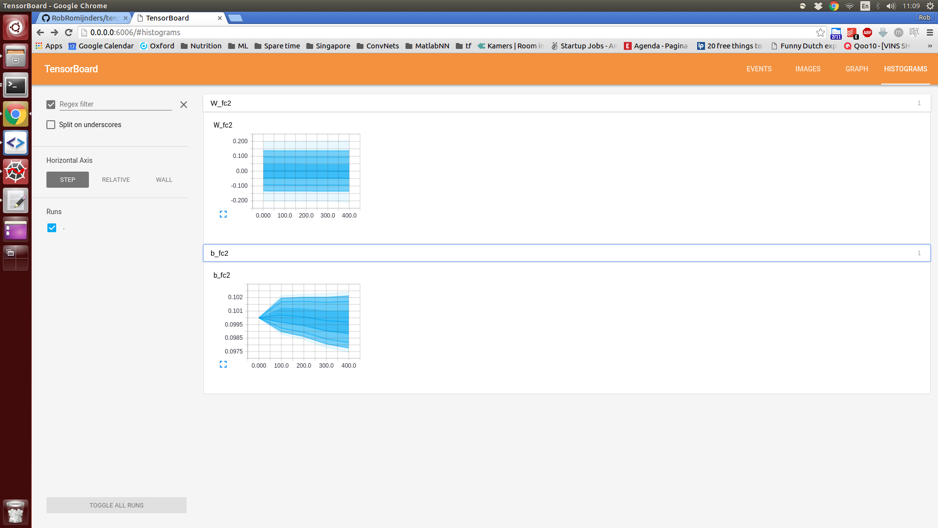
# Also add histograms to TensorBoard
w_hist = tf.histogram_summary("W_fc2", W_fc2)
b_hist = tf.histogram_summary("b_fc2", b_fc2)

with tf.name_scope("Entropy") as scope:
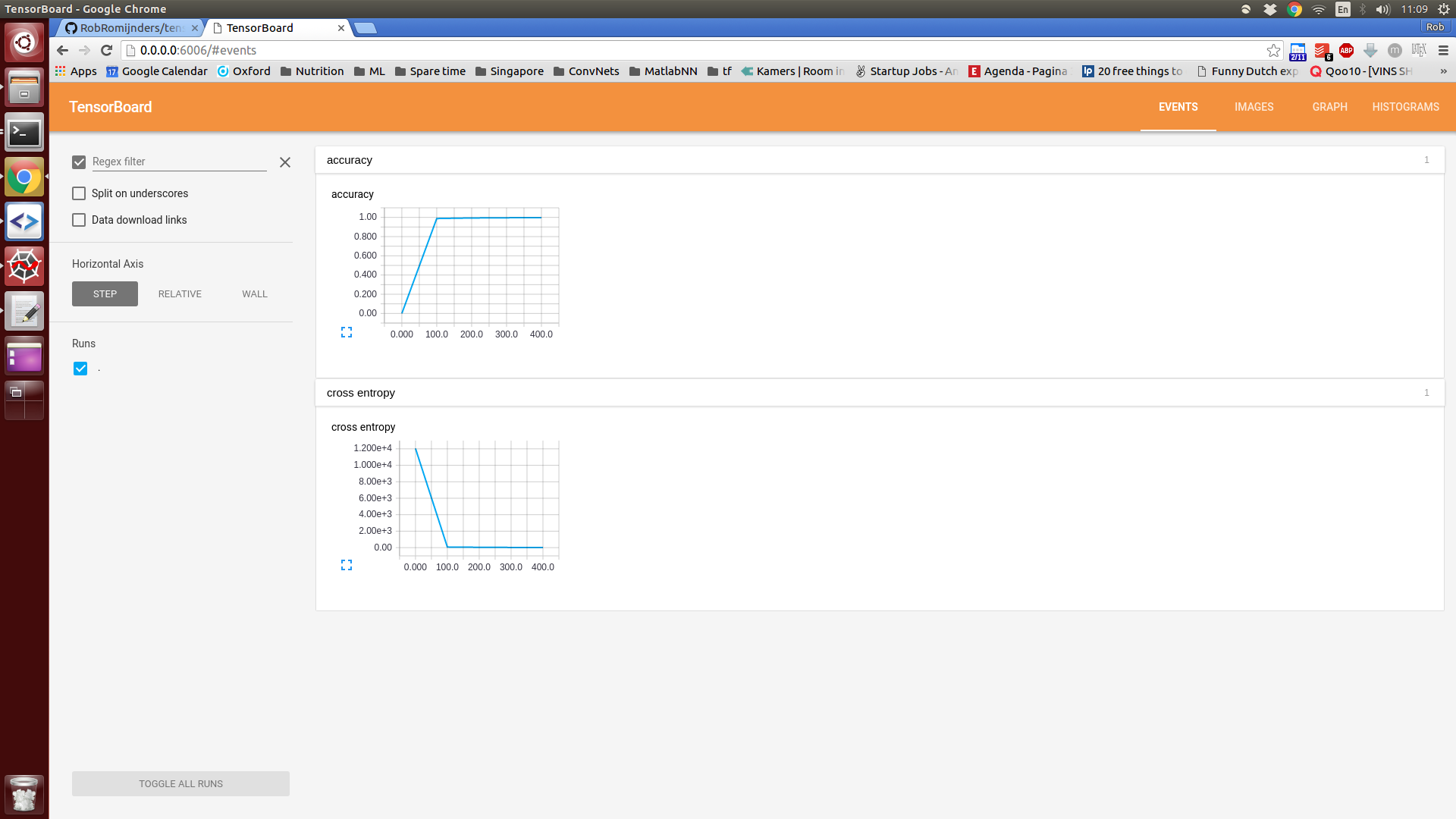
    cross_entropy = -tf.reduce_sum(y_*tf.log(y_conv))
    ce_summ = tf.scalar_summary("cross entropy", cross_entropy)
with tf.name_scope("train") as scope:
    train_step = tf.train.AdamOptimizer(1e-4).minimize(cross_entropy)
with tf.name_scope("Evaluating") as scope:
    correct_prediction = tf.equal(tf.argmax(y_conv,1), tf.argmax(y_,1))
    accuracy = tf.reduce_mean(tf.cast(correct_prediction, "float"))
    accuracy_summary = tf.scalar_summary("accuracy", accuracy)


merged = tf.merge_all_summaries()
writer = tf.train.SummaryWriter("/home/rob/Dropbox/ConvNets/tf/log_tb", sess.graph_def)

sess.run(tf.initialize_all_variables())
for i in range(500):
  batch_ind = np.random.choice(N,50,replace=False)
  if i%100 == 0:
    result = sess.run([accuracy,merged], feed_dict={ x: X_test, y_: y_test, keep_prob: 1.0})
    acc = result[0]
    summary_str = result[1]
    writer.add_summary(summary_str, i)
    writer.flush()  #Don't forget this command! It makes sure Python writes the summaries to the log-file
    print("Accuracy at step %s: %s" % (i, acc))

  sess.run(train_step,feed_dict={x:X_train[batch_ind], y_: y_train[batch_ind], keep_prob: 0.5})

sess.close()

# We can now open TensorBoard. Run the following line from your terminal
# tensorboard --logdir=/home/rob/Dropbox/ConvNets/tf/log_tb